


 English (pdf)
 Article in xml format
 Article references
 Send this article by e-mail
 Cited by SciELO
  Similars in
SciELO
Similars in
SciELO 
 Permalink
I. Introduction
In the Brazilian Amazon region, rivers and their tributaries contain an extensive floodplain that corresponds to approximately 12% of the humid area of the Amazon basin. These floodplains present enormous terrestrial and aquatic biodiversity (Melack & Hess, 2010). Accurate flood monitoring not only in the Brazilian Amazon but also other regions of the world is important for increasing the security of local inhabitants and for reducing infrastructure damages and income losses. Besides, the frequency and magnitude of flood events are expected to increase due to climate change.
Flood monitoring can be conducted based on satellite observations, because of their ability to cover large areas, at high repetition and low costs. Inundation detection has been addressed based on several optical satellites (e.g., Landsat, Sentinel-2, and Moderate Resolution Imaging Spectroradiometer onboard Terra and Aqua platforms) operating at different spatial, spectral, and temporal resolutions. They exploit the high level of absorption of radiation incident into the water bodies in the near-infrared and shortwave infrared spectra relative to the visible spectrum. However, the Amazon tropical region faces persistent cloud cover conditions most of the year, making the use of optical remote sensing data limited.
Synthetic Aperture Radar (SAR) remote sensing can be an important source of information for mapping flooded areas in the Brazilian Amazon because of its ability to acquire images under cloud-covered conditions. SAR sensors can identify inundation because of the typically lower backscattering returns from water bodies relative to other features. Basically, flooded areas in single SAR images are discriminated from non-flooded areas by thresholding backscatter values at different polarizations (Matgen et al., 2011), subtracting backscattering coefficients between two images (Schlaffer et al., 2015), or calculating variance in time series (DeVries et al., 2020).
More recently, machine learning (ML) and deep learning (DL) classifiers are becoming quite popular in the field of remote sensing image classification. Although there is an overall agreement that DL is more powerful than ML, it requires bigger computational capabilities and so it may not be operational for studies involving large areas such as the Brazilian Amazon. ML-based image classification can be divided into supervised, unsupervised, and reinforcement learning categories. The two most used supervised ML classifiers are the Random Forest (RF) and Support Vector Machine (SVM) because they usually provide high accuracies in different types of land use and land cover classifications, including flooded and non-flooded classes (Banks et al., 2019; Millard & Richardson, 2013; Mohammadimanesh et al., 2018). The other popular supervised algorithms include naive Bayes and neural networks (Acharya et al., 2019; Boateng et al., 2020; Nemni et al., 2020). Several authors have reported that divergences in the classification results can be substantial due to the differences in sensor systems, timing, and data processing algorithms (e.g., Aires et al., 2013; Pham-Duc et al., 2017; Rosenqvist et al., 2020).
This study aims to evaluate the potential of the Artificial Neural Network Multi-Layer Perceptron (ANN-MLP) and two k-Nearest Neighbor (KNNs) algorithms to delineate flooded areas in a stretch of the Amazonas River in Central Amazon using Sentinel-1 SAR time series from 2017, 2018, and 2019. To our best knowledge, there is no study evaluating these ML classifiers to identify flooded areas in the Brazilian Amazon, especially using Sentinel-1 SAR data sets. Among the 29 studies listed recently by Fleischmann et al. (2022) involving inundation mapping by remote sensing over the Brazilian Amazon, nine relied on SAR data, all acquired by the ALOS/PALSAR mission. Currently, the only SAR data freely available on the internet are the ones acquired by the European Space Agency (ESA) Sentinel-1 satellite (Torres et al., 2012). We addressed the following research question in this study: what are the performances of the ANN-MLP and KNN-based ML algorithms to map flooded areas in tropical rainforests based on Sentinel-1 satellite data?
II. Materials and methods
1. Study area
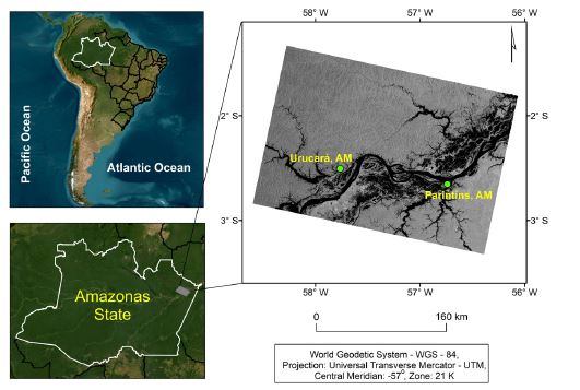
The study area is located between the municipalities of Urucará and Parintins in the Amazonas State, Brazil, comprising part of the Amazonas River. It is located between the following coordinates: 22°30′48.84″ and 22°37′59.16″ of south latitude; and 44°31′35.68″ and 44°43′25.94″ of west longitude (fig. 1). The typical climate is classified as Af, that is, tropical rainforest climate without dry season, in the Köppen′s classification system, with average annual precipitation ranging from 1355mm to 2839mm (Alvares et al., 2014). The average annual temperature varies from 25.6°C to 27.6°C. The flooding period occurs mostly between May and July.
2. Remote sensing data sets
This research used three Sentinel-1 SAR images acquired in the VV and VH polarizations during the following flooding periods: 23 June 2017; 18 June 2018; and 7 July 2019. The images were obtained in descending, Interferometric Wide (IW) mode, and processed at Level-1, which includes pre-processing and data calibration (table I).
Table I Sentinel-1 SAR image acquisition modes.
| Mode* | Incident Angle (º) | Spatial Resolution | Swath Width (km) | Polarization |
|---|---|---|---|---|
| SM | 20° − 45° | 5m×5m | 80 | HH or VV or (HH and HV) or (VV and VH) |
| IW | 29° − 46° | 5m×20m | 250 | HH or VV or (HH and HV) or (VV and VH) |
| EW | 19° − 47° | 20m×40m | 400 | HH or VV or (HH and HV) or (VV and VH) |
| WV | 22° − 35° 35° − 38° | 5m×5m | 20 | HH or VV |
* SM = StripMap; IW = Interferometric Wide; EW = Extra Wide; and WV = Wave.
Source: ESA (2017)
We also selected Sentinel-2 MultiSpectral Instrument (MSI) images acquired near the Sentinel-1 SAR overpasses (2 July 2017; 22 June 2018; and 29 July 2019). In this study, the Sentinel-2 was used to collect sampling data for training, validation, and testing. The Sentinel-2 MSI images were radiometrically corrected. They have the potential for mapping flooded areas at regional scales, as they are acquired under the spatial resolutions of 10m to 60m and temporal resolution of 10-days (Du et al., 2018) (table II).
3. Methodological approach
Figure 2 shows the main steps of the methodological approach used in this study. We conducted the following pre-processing steps: correction by the orbit file; terrain correction; radiometric calibration; conversion of the data to decibels; and spatial filtering. The images were pre-processed by the image orbit file, containing accurate information on the satellite´s position, trajectory and speed during the image capture process (ESA, 2017). The terrain correction was based on the digital elevation model (DEM) acquired by the Shuttle Radar Topographic Mission (SRTM) at ~3 arc sec-1. The radiometric calibration was performed using the Sigma Look-Up Table (LUT) file to generate images converted into backscattering coefficients (σ0).
SAR images present speckles that originate from destructive or additive interference from the radar return signal for each pixel (Lee & Pottier, 2009). We used Lee filter with a 3×3 window size for processing VV- and VH-polarized images. The Lee filter transforms the multiplicative model into an additive model by expanding the first-order Taylor series around the average. This technique uses local statistics to minimize the mean square error (MSE) through the Wiener filter. In this way, the Lee filter is an adaptive filter that has the characteristics of preserving edges (Sant'Anna, 1995). Lee's filter assumes that the mean and variance of the pixel of interest are equal to the mean and variance of all local pixels, which refer to the inside of the adopted window.
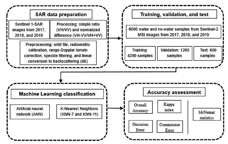
Fig. 2 Methodological flowchart with the main steps for classifying flooding areas in the Central Amazon in 2017, 2018, and 2019.
We used the following image processing software: S1-Toolbox available in the Sentinel Application Platform (SNAP) version 7.0.0; ArcGIS version 10.5; and Abilius, which uses the OpenCV library of artificial intelligence algorithms in the C++ programming language.
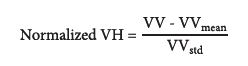
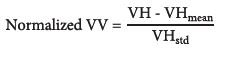
Sentinel-1 images converted into backscattering coefficients were normalized based on their averages and standard deviations (eq. 1 and 2).
 ***
***
 ***
***
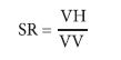
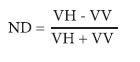
The normalized images were also processed to generate the simple ratio (SR) index and normalized difference (ND) index involving VH and VV polarizations (Hird et al., 2017; Tsyganskaya et al., 2018) (eq. 3 and 4).
 ***
***
 ***
***
As pointed out by Boateng et al. (2020), the most widely used nonparametric ML techniques include ensembles of classification trees such as Random Forest (RF) (Breiman, 2001), Artificial Neural Networks (ANNs) (Brown et al., 2000), K-Nearest-Neighbors (KNN) (Breiman & Ihaka, 1984), Support Vector Machines (SVMs) (Cortes & Vapnik, 1995). In this study, we selected two classifiers, the ANN and two KNN (KNN-7 and KNN-11) algorithms to verify the performance of these techniques to classify flooded areas in the region of interest. The widely used RF classifier was not selected because we are interested in only two classes (water and non-water), making it impossible to develop a random forest, ensemble architecture that is the basis of these algorithms. In this ensemble architecture, several classification trees are trained based on subsets of the training data (Abdi, 2020). We did not evaluate SVM either because, together with RF, it has been intensively assessed in literature over several different environmental and terrain conditions.
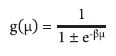
The ANN adopted in this study was the Multilayer Perceptron (MLP) type with the backpropagation learning algorithm with insertion of the momentum term, which optimizes the network processing with a learning rate of 0.05 and a momentum factor of 0.5. According to Atkinson and Tatnall (1997), there are several advantages of neural networks, such as the efficient manipulation of large data sets and their use in the classification of remote sensing data without assuming a normal distribution. In the classification by neural networks, we used the Abilius program developed by the University of Brasília, Brazil, which is based on the OpenCV library. We used the logistical activation function in which the output result of the neuron, given a set of input signals, assumes real values between zero and one to facilitate the network training process and to simplify its structure (eq. 5):
 ***
***
where β = real constant associated with a slope level of the logistic function related to its inflection point; and µ = activation potential produced by the difference in value produced between the linear combination and activation threshold.
The KNN classifier is a non-parametric method based on k-training samples closest to the behavior of the analyzed data (Cover & Hart, 1967). The calculation of the nearest neighbor was performed using the Euclidean distance method. In this classification technique, the k-value refers to the number of neighbors to be used in determining the class assigned by the values of most of the nearest pixels that must be assigned. There are several studies in the literature with different values of k (Alves et al., 2013). The unknown sample is assigned to the most common class of the k-training samples that are nearest in the feature space to the unknown sample (Maxwell et al., 2018). In this study, we assigned k-values of seven and eleven. These numbers are a compromise between too-low and too-high k-values. Low k-values will produce complex decision boundaries while high k-values will result in greater generalization (Maxwell et al., 2018).
The training, validation, and testing data set was produced by manual sample collection of 6000 pixels (denoized time signatures) containing two classes (water and non-water), with equal distribution (3000 samples per class), showing well-distributed sampling design (fig. 3). We considered a total of 4200-pixel samples for training (70%), 1200-pixel samples for validation (20%) and 600-pixel samples for testing (10%), according to the methodology defined by Kuhn and Johnson (2013) and Larose and Larose (2014). The training of ANNs considered different architectures for VV, VH, SR, and ND images. The number of neurons in the hidden layer was determined by the trial and error methods (Hirose et al., 1991). The selected stopping criterion was the number of learning cycles, defined as 10 000. At the end of the training process, 180 sets of independent samples were collected to validate the classification results. The selection of the best classifier was based on the lowest values of mean squared error (MSE).
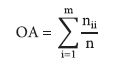
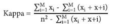
The accuracy of the classification was analyzed using the confusion matrix, omission and commission errors, overall accuracy, and Kappa index (Congalton & Green, 1993). Overall accuracy (OA) and the Kappa index were calculated using equations 6 and 7:
 ***
***
where n ii = diagonal elements of the confusion matrix; n = total number of observations; and m= number of themes mapped.
 ***
***
where n = total number of observations; and x i and x+i are the sums in row and column.
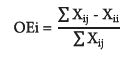
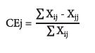
Kappa is a coefficient that varies from zero to one, representing a general agreement index. Kappa values are associated with the quality of the classification. Cell values were considered for measuring omission and commission errors. The marginal cells in the lines indicate the number of pixels that were not included in a particular category, that is, express the error known by default. Cells on the diagonals represent the pixels that were not included in no category, expressing the error of commission (Congalton & Green, 1993). The omission error (OEi) and the commission error (CEj) were calculated for the thematic classes of the classification (eq. 8 and 9):
 ***
***
 ***
***
where ΣX ij - X ii = sum of waste per line; ΣX ii - X jj = sum of waste per column; and ΣX jj = row or column marginal.
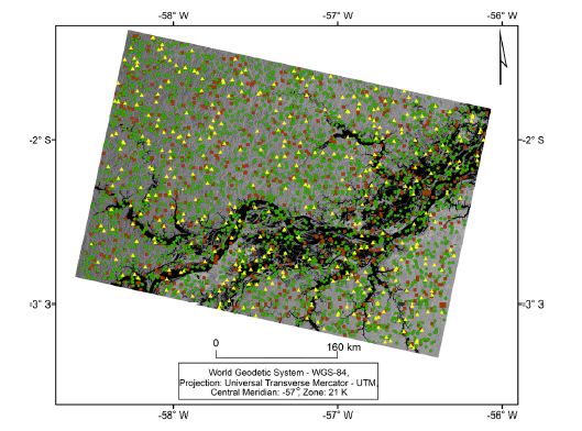
Fig. 3 Location of the samples for training (green circle), validation (brown square), and test (yellow triangle).
We also conducted another validation strategy based on the Sentinel-2 MSI scenes from June and July of 2019 and the McNemar chi-squared test (2). The accuracy analysis used 88 systematic samplings with a 10km diameter in regular grids of 17×17km2 (fig. 4). We disregarded the cloud-covered samples in the Sentinel-2 images.
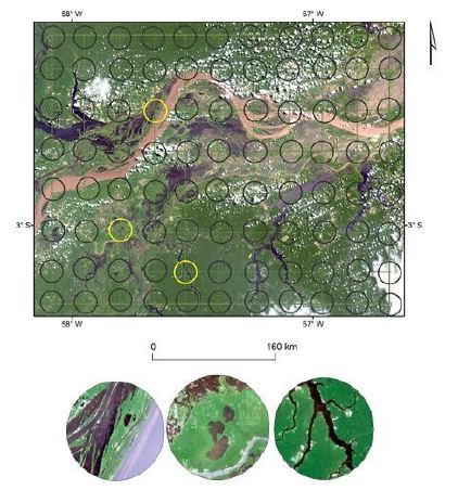
Fig. 4 Location of systematic samples for validation of flooding maps produced by the machine learning classifiers.
McNemar’s 2 test was used considering a statistical level of significance of 0.05 and one degree of freedom to analyze the differences in measured areas between visual interpretation and classified images. According to McNemar (1947) and Leeuw et al. (2006), McNemar's analysis is a non-parametric statistical test to analyze pairs and has been widely used in remote detection because it can use the same validation set (Eq. 10):
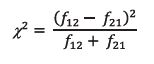 ***
***
where f 12 = number of wrong classifications by Method-1, but correctly classified by Method-2; and f 21 = number of correct classifications correct by Method-1, but incorrectly classified by Method-2.
This precision comparison based on related samples is quite popular in the literature (Abdi et al., 2020; Manandhar et al., 2009; Mayer et al., 2021; Wang et al., 2018). The McNemar statistical test was performed at the level of significance of 0.05 and one degree of freedom between the image classifiers to analyze whether the classified images differ statistically.
III. Results
1. Backscattering values of flooded areas
Table III presents the statistical results for the backscatter coefficients of the three-year images in dual polarization from the Sentinel-1 SAR satellite before and after the data normalization. The results of the normalization showed a slight increase in the mean values compared to the non-normalized images. The value of variance and standard deviation remained identical with the image before adjustment. Decreasing mean values in the fitted images represents a greater concentration of the distribution data, compressing the backscatter values for the image. In other words, the decrease in the mean and standard deviation values indicates a low dispersion of the backscattered data. The characteristics and multi-temporal patterns of the backscatter values were similar to the VH and VV polarizations, as well as to the SR and ND images for the three years.
Table III Statistical results before and after normalization of Sentinel-1 SAR images from 2017 to 2019.
| Overpass | Normalization | Mean VH | Mean VV | Standard Deviation VH | Standard Deviation VV | Variance VH | Variance VV |
|---|---|---|---|---|---|---|---|
| 23 June 2017 | Non-normalized | -10.68 | -7.08 | 8.77 | 7.14 | 76.91 | 50.97 |
| Normalized | -9.46 | -6.09 | 8.77 | 7.14 | 76.91 | 50.97 | |
| 12 July 2018 | Non-normalized | -9.96 | -6.29 | 7.69 | 5.76 | 59.13 | 33.17 |
| Normalized | -8.67 | -5.20 | 7.69 | 5.76 | 59.13 | 33.17 | |
| 17 June 2019 | Non-normalized | -10.50 | -6.63 | 7.86 | 5.93 | 61.77 | 35.16 |
| Normalized | -9.16 | -5.52 | 7.86 | 5.93 | 61.77 | 35.16 |
Figure 5 shows the box plot in a range of grouped multi-temporal backscatter values, measured in all scenes (VH, VV, SR, and ND). In comparison to the backscatter values of water bodies in the time series, there was a considerable increase in the average backscatter values in the following order: VH, VV, SR, and ND. The backscatter of water bodies in the VH image was the lowest among the three scenes, with an average value of -25.8dB in the upper limit and -20.0dB in the lower limit and with backscattering in the value of -24.2dB in the first quartile. In contrast, the VV polarization presented the largest data series between the lower and upper limits, with the upper limit lower value at -23.3dB and the upper limit at -13.3dB, with 75% of its backscatter values being represented by -15.8dB, as shown in quartile-3.
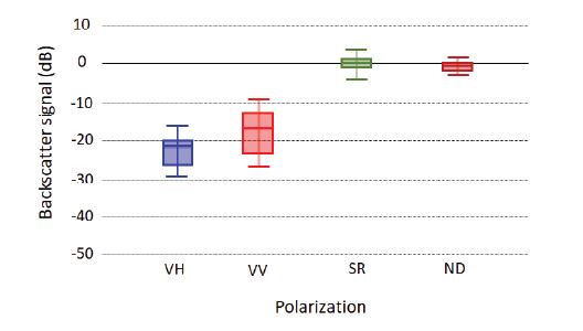
Fig. 5 VH, VV, SR and ND backscatter values over water bodies obtained by averaging the Sentinel-1 scenes from 2017, 2018, and 2019.
The VH polarization showed the lowest backscatter values for the water body due to the record of the backscattered value of the return signal on the antenna occurring in the horizontal direction. The backscatter values of the indices became more aggregated compared to the scalar values of the polarizations VH and VV, with median, quartiles, and closest limits for the index images.
2. Best ANN model for flooded area detection
The ANN model with the combination of VV and VH polarizations as well as SR and ND presented accurate results in the network learning and training tests, with: 91.3% and 91.9% of overall accuracies for the image acquired in 2017; 90.7% and 90.9% accuracies for 2018; and 90.2% and 90.7% accuracies for 2019. The ANN architecture with the best results was obtained using four neurons in the input layer, two hidden inner layers with eight neurons, and two neurons in the output layer (4-8-8-2 model) (fig. 6).
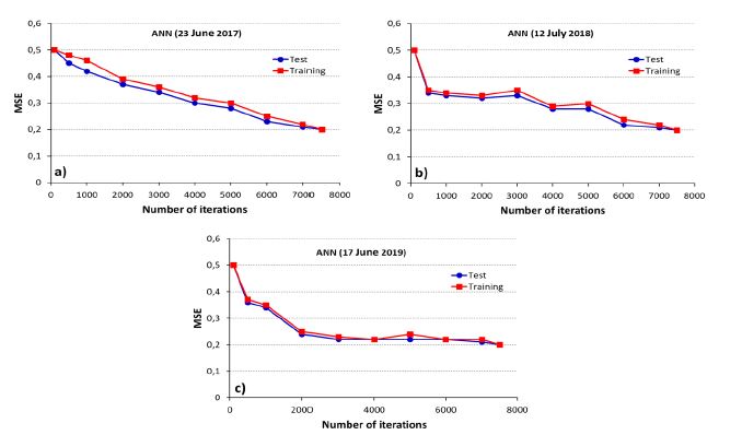
In the learning phase of the three ANNs, the training errors were slightly higher than the test errors. However, with the increasing number of trainings in some moments, these errors were equalized. The errors stabilized with values of root mean square error (RMSE) in 0.2. The maximum cycles did not exceed 10 000 iterations. These values demonstrate that the maximum learning limit of ANN with 10 000 iterations is sufficient for training, which results in high precision, accuracy, and lower computational processing cost (fig. 7).
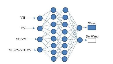
Fig. 6 The most appropriate artificial neural network model for classifying water bodies in the study area (4-8-8-2).
3. Classification results
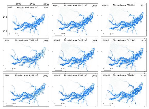
Figure 8 shows the classification of the flooded areas in the Central Amazon region using the ANN, KNN-7, and KNN-11 classifiers in the period of largest flood pulse during the years 2017, 2018, and 2019. The blue-colored areas correspond to areas classified as water bodies. The classifiers delimited precisely the main channel of the Amazon River, as well as the flooded areas adjacent to the river channel. In general, the classification through ANN generated products classified with slightly higher clarity when compared to the KNN classifiers.
The noises classified as upper lands increased from KNN-7 to KNN-11, indicating that the increase in the Euclidean distance from seven to eleven contributes to the increase of confusion between the water body and the upper land. In addition, there was a misclassification of water bodies for all images. These areas are shown as random blue dots mainly after the boundary of the tributaries of the Amazon River, as well as the presence of random pixels scattered in various regions spread in the entire study area.
The largest presence of water bodies was found in the image acquired in 2019, with a total area of 6244km² (ANN), 6268km² (KNN-7), and 6290km² (KNN-11). In other words, the KNN-7 and KNN-11 algorithms presented the largest occurrences of water bodies, as compared with the ANN classification.
4. Accuracy analysis
The image classification by ML showed Kappa coefficient values from 0.77 to 0.91 (table IV). ANN showed higher accuracy for all Sentinel-1 scenes. Second in the classification order, the KNN-7 presented results close to the ANN. The KNN-11, on the other hand, presented the highest differences in the accuracies among the three classifiers, obtaining the lowest Kappa index (0.77) in the image acquired in 2018.
There was no discrepancy between Kappa indexes and the overall accuracies. The classifications by ML showed high overall accuracy values, with ANN presenting the highest values, with 97% in the image from 2019. The lowest value was presented by KNN-11, with 92%, in the image acquired in 2018.
Table IV Kappa coefficient, overall accuracy, and omission and commission errors in the SAR images processed by the ANN, KNN-7, and KNN-11 classifiers.
| Satellite Overpass | Kappa | Overall Accuracy (%) | Commission Error (%) | Omission Error (%) |
|---|---|---|---|---|
| ANN | ||||
| 23 June 2017 | 0.87 | 96 | 8.99 | 2.99 |
| 12 July 2018 | 0.85 | 93 | 10.90 | 3.98 |
| 17 June 2019 | 0.91 | 97 | 6.99 | 1.99 |
| KNN-7 | ||||
| 23 June 2017 | 0.85 | 95 | 10.9 | 4.9 |
| 12 July 2018 | 0.82 | 95 | 12.9 | 5.9 |
| 17 June 2019 | 0.88 | 96 | 8.99 | 3.9 |
| KNN-11 | ||||
| 23 June 2017 | 0.83 | 94 | 17.9 | 8.9 |
| 12 July 2018 | 0.77 | 92 | 18.9 | 12.9 |
| 17 June 2019 | 0.85 | 95 | 11.5 | 5.7 |
The ANN classification technique obtained the lowest commission error, with 7.0% and omission error of 1.9%, in the image from 2019. The largest commission and omission errors were measured in the image from 2018, classified by KNN-11, with a commission error of 18.9% and an omission of 12.9%. There was more commission error when compared to the omission error in all products generated by the classifiers, proving that the biggest classifier errors occurred in the definition of the drylands as the water body.
The image from 2018 was measured with the lowest presence of water bodies, which was also the image that presented the largest errors and the worst statistical indices analyzed. Thus, it is inferred that due to the smaller grouping and the greater distance between the pixels corresponding to the backscatter values of the water bodies was the determining factor for obtaining the worst results obtained by the KNN classifier with Euclidean distance of eleven.
The classifiers produced an overall good performance in delineating water bodies, especially the ANN and the KNN-7. They showed the lowest levels of noise in the images (fig. 9). The results of the indexes showed that the ANN obtains the best performance in comparison with the other classifiers. ANN and KNN-7 achieved similar levels of precision in two of the three images, these images being classified with greater quantities of water bodies. On the other hand, it was observed that the worst indices occurred in the KNN-11 classification and were obtained in the image with the least amount of water bodies.
Table V shows the results of the McNemar test between the pairs of the three classifications, considering the different combinations of parameters. The ANN showed the best results in the time series, despite obtaining the best values between the methods. The ANN did not differ statistically from the KNN-7 classifier in the time-period. The KNN-11 classifier presented the highest value of χ² with 4.37, in the image from 2018. This result was statistically significant, rejecting the hypothesis of statistical equality between the pairs of classifiers RNA × KNN-11 at the p-value of 0.05, since the calculated χ² is higher than the tabulated χ² (3.84).
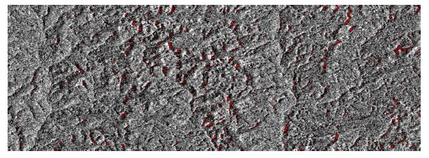
In general, the biggest confusion for image classifiers was to distinguish the water class from other non-water targets with similar backscatter values. In this way, the presence of the shadow effects was observed in all images, indicating that this effect was the biggest cause of misclassification, with less interference only in ANN classification (fig. 10).
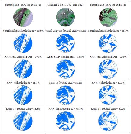
Fig. 9 Results of visual interpretation (Sentinel-2) and Machine Learning (ML) classification (Sentinel-1) of three enlarged images acquired in 2019.
Table V McNemar test between visual interpretation and ANN, KNN-7, and KNN-11 classifiers shown in terms of χ² values.
| Sentinel-1 Overpass | Visual × ANN | Visual × KNN-7 | Visual × KNN-11 | ANN × KNN-7 | ANN × KNN-11 | KNN-7 × KNN-11 |
|---|---|---|---|---|---|---|
| 23 June 2017 | 2.10 | 2.36 | 3.63 | 2.64 | 2.94 | 2.86 |
| 12 July 2018 | 2.30 | 3.61 | 4.28(*) | 2.98 | 4.37(*) | 2.77 |
| 17 June 2019 | 2.68 | 3.55 | 4.46(*) | 2.12 | 2.53 | 2.36 |
(*) represents statistical significance, with the calculated value of χ² greater than the tabulated value at a significance level of 5% (3.84).
IV. Discussion
The C-band backscattering coefficients of flooded areas in 2017, 2018, and 2019 varied from -10.68dB to -9.96dB in the VH polarization and from -7.08dB to -6.29dB in the VV polarization in the study area. These values are quite higher than those found by Magalhães et al. (2022) for open water bodies in the Amazon River: -19dB in the VH polarization and -14dB in the VV polarization. Conde and Muñoz (2019) reported that backscattering intensity values of permanent water bodies are below -20dB. Moharrami et al. (2021) applied a threshold value of -14.9dB to the Sentinel-1 scenes to delineate flooded areas. Our higher values are probably due to the contribution of sparse shrubs and trees that we find in flooding areas in the surface backscattering process.
The accuracy assessment based on Kappa index, omission and commission errors showed overall accuracies of detecting flooded areas close to one another and higher than 90% for all three classifiers. These values are comparable to or higher than the accuracies obtained by other scientists who used Sentinel-1 SAR data for classifying flooded areas around the world. For example, Twele et al. (2016) used a processing chain approach to detect flood conditions in two test sites at the border between Greece and Turkey. They showed encouraging overall accuracies between 94.0% and 96.1%. Liang and Liu (2020), in their water and non-water delineation study using four different thresholding methods, reached overall accuracies ranging from 97.9% to 98.9% for a study area located in Louisiana State, USA. Siddique et al. (2022) evaluated RF and KNN algorithms applied to Sentinel-1 images from North India and concluded that C-band SAR data can detect changes in flood patterns over different land cover types with overall accuracies ranging from 80.8% to 89.8%.
The comparison between visual analysis and the selected ML classifiers based on three enlarged images (fig. 9) showed an overall underestimation of flooded areas for the ML classifiers. However, the NcNemar 2 test showed that the results from visual interpretation and ML classifiers were statistically equal from each other. The only exceptions were found for the KNN-11 applied in the scenes acquired in 2018 and 2019. The McNemar test also showed that ANN x KNN-7 and ANN x KNN-11 did not differ statistically each other. These results indicate the existence of site-specific spatial heterogeneity within the study area. In other words, the overall statistical results found for the entire study area may differ depending on the local landscape conditions within the study area.
Figure 10 showed the presence of shadowing effects in the flood delineation, leading to higher commission errors. This effect has been reported widely in the literature (e.g., Chen & Zhao, 2022), even sometimes its presence in SAR images is used as an indicator of some targets, mainly deforestation (Bouvet et al., 2018). Shadowing effects occur in SAR images because of their mandatory side-looking geometry. In other words, shadows in SAR images are related to areas in the terrain that cannot be reached by emitted radar pulses. As Sentinel-1 scenes are acquired in an almost north-south orbit (98.2° of inclination), most of the pixels classified as flooded in the upper lands are also oriented approximately north-south.
V. Conclusion
The Sentinel-1 SAR images classified by ML algorithms showed good potential to map flooded areas in the Central Amazon. The three tested algorithms produced accuracies ranging from 92% to 97%. ANN and KNN-7 classifiers showed better potential than the KNN-11. Shadow effects appearing in non-flooded areas surrounding the flooded areas increased the commission errors.
The methodological approach used in this study may be suitable to map flooding areas in other regions of the Brazilian Amazon, but no broader generalizations can be made as the performance of the methods varies according to the local environmental and biophysical conditions.
As SAR images are quite sensitive to texture, the addition of textural attributes derived, for example, from the Gray Level Co-occurrence Matrix (GLCM), such as the angular second moment, dissimilarity, entropy, and variance in the classification procedure may improve the classification results. More recent studies have demonstrated the high performance of DL algorithms so they also should be tested to map flooded areas. U-Net and tensor flow are the ones that are becoming quite popular in the DL group of classifiers.
Acknowledgements
The authors are grateful for financial support from CNPq. Special thanks to the research groups of the Laboratory of Spatial Information System at the University of Brasilia. Finally, the authors thank the anonymous reviewers who improved this research.
Authors' contributions
Ivo Augusto Lopes Magalhães: Conceptualization; Methodology; Software; Validation; Formal analysis; Research; Writing. Osmar Abílio de Carvalho Júnior: Conceptualization; Methodology; Software; Resources; revision and editing; Visualization; Supervision; Fund acquisition. Edson Eyji Sano: Methodology; Validation; Data curation; Writing - revision and editing; Visualization.

